Previous Example    Next Example

Fitting a mathematical model to match the experimental data falls in the domain of parameter estimation. It is of particular practical importance when parameters are difficult to measure directly. To illustrate this fascinating subject let's modify the optimal trajectory example for the purpose of estimating the coefficient of drag from the measured trajectory data.

The algorithm steps can be informally sketched with a pseudo-code,

<INIT>   Initialize equations of motion

               do while ( not_end_of_file )
                  integrate (eom)
               end do

               if ( obj_fcn  >  criteria ) then
                  estimate (Cd)
                  go to  <INIT>
               end if

Except for the manipulation of measured data imported to the simulation model, the solution is notably similar to the previous case.

      if(init()) open(85,file='meas_trj.dat')
      call estimate (iest,isim,m,n,Cd,range,tol,pif)
      if(isim .eq. 1) call oprtn                 ! start simulation

      if(mode() .eq. initialize) then                     
        dist   = 0
        height = 0
        vx     = v0*cos(alfa)
        vy     = v0*sin(alfa)
      endif

*        Define & integrate eom
      vsq  =  vx**2 + vy**2
      Drag = .5*Cd*Ap*rho(height)*vsq
      alfa =  atan(vy/vx)

      dx(1) =  vx
      dx(2) = -(Drag/mass)*cos(alfa)
      dx(3) =  vy
      dx(4) = -(Drag/mass)*sin(alfa) - g

      call integral (mode(),dt(),4,S,id,dmy,dmy,x,dx)
*
      if(sched(tk)) then                    ! reset on eof
        read(85,*,iostat=status) hm_tk
        if(status .eq. eof) then
          rewind 85
          isim = 0 
          call icrtn
        else
          pif = obj_fcn (height,hm_tk)
        endif
      endif

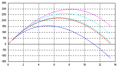
A noteworthy difference appears in the "termination block" which is synchronized with the data sampling instants of the measurements stored in the file. The simulation runs are repeated automatically until the estimated parameter Cd is within prescribed tolerance. i.e. until the area (calculated by obj_fcn) between measured and calculated trajectories is minimized.

Trajectory (height vs. time) marked in red corresponds to the final parameter
estimate - a perfect fit due to noiseless measurements.

A straightforward transition from the optimal trajectory setup to parameter estimation is largely due to native file data handling capabilities. The operational differences are reflected in the graph showing trial trajectories which are now of the same duration.